A long and winding R0(ad)1

It's an unbelievable relief that, two weeks ago, I got an official email from my (very supportive) program officer at the NCI letting me know that my first R01 was going forward for funding. In celebration of this, I want to do convey three things.

1 - The science we are going to do!
2 - The long road of rejections (and necessary improvements) leading up to this (persistence pays off)
3 - How grateful I am to the many, many people who were involved along the way.

I'm going to convey these in opposite order...

3 - Gratitude:

It wasn't just me working on my own... on the contrary, this was a process that began during my scientific training where my mentors let me read/edit their grants, read/edit manuscripts, and yes, write my own. It was gracious colleagues reading my drafts, editing my aims, discussing the science with me. It was people betting on me by giving me a job and startup...  joining our lab team before we were funded. It was family and friends listening to me rant after rejections.  And of course, scientific collaborators working as hard and long as I did (looking at you Andriy). So, first order of business: thanks!

2 - Long and winding (painful) road.

This particular grant, which I will describe in the next section, was not, by any means, funded on the first try. In fact, it took about 4 years... and 6 submissions. 
Three R21s: one scored (*8*, 4, 3), a resubmission not discussed, and a new submission after that not discussed.
Then three submissions of R01s: 21% (3, 4, 5), 17% (3, 4, 4) and finally the awarded grant (which was 10% (2, 2, 4)).

Some takeaway thoughts about this.

Many of the ideas were the same (not all) -- those which the study section liked, I kept -- those they didn't, I rethought. For the most part, while I was frustrated and sometimes even angry at my rejections, but upon further reflection I usually found that their opinions were pretty well founded.

In hindsight, I'm also sort of amazed how immature the ideas I originally submitted were. While the ideas were sound (for the most part), the data wasn't there to support any of my claims.  Here is an example from the first R21 submission in 2016, side by side with one from the funded R01 in 2019 (almost 2020). You can see on the left some 'background' where I suggest the experiment I WANT to do...  then, we did it, and analyzed it, and published it (1.5 years later), and it became a subpanel of 'previous work' in the funded proposal (right).

Left: an idea of what a collateraa sensitivity matrix MIGHT look like after the experiments I posed (yes, i made that with powerpoint). Right (panel A), what it looks like now as preliminary data...  and B-F some more interesting observations from those (now published) experiments -- see Dhawan et al.

Another interesting tidbit.  After getting back my first R01 score (21%), I was able to take advantage of the 'quick turnaround resubmit' for ESIs (now defunct), so only had a few weeks to get it back in.  This meant that I could only really address small issues the reviewers had. In this case, I was able to add a co-authored publication with a new method for comparing in vivo growth curves, but not much else except a small in vivo experiment Andriy has performed (which has since been expanded into a whole paper on its own showing the graduality of the evolution of resistance -- which in turned has spawned a new grant -- this one still in the infant stages of development).  Changing out the aim that was the big sticking point wasn't possible though on the short timescale. I was frustrated by the result (but maybe shouldn't have been surprised), and got a 17% on the A1.

17% is pretty far outside the funding range, but the PO was very supportive, and presented it for exception.  At the end, it wasn't funded, but I was very encouraged by the support.  TALK TO YOUR PROGRAM OFFICERS!

So, with more time, and the new summary statement, I was able to thoughtfully rewrite a new A0, which included two new publications (the EGT one from above, and our collateral sensitivity/experimental evolution work in E. coli, both of which I've blogged about here before (road to measuring evolutionary game in cancer and Antibiotic collateral sensitivity is contingent on the repeatability of evolution). Cynically, one could say it was the two 'shiny' journals we published in that put us over the edge, which is likely in part true, but I think it was much more the honing of the science and grantspersonship that we managed.

Anyways, happy to share any/all of the grants/summary statements if you want to learn from my mistakes, just shoot me an email.

Right. Now the science (in blog/tweetorial format - which I will cross-post on the mathoncoblog):

my third attempt at this R01 submission that went to MABS - scores went A0: 21%, A1: 17%, rewritten new A0: 10% (funded through magic of ESI thank you @NIHFunding)  #persistence

we are excited to study the evolution of TKI resistance in lungcancer - through three specific aims:

Together with @AndriyMarusyk our first aim will be to see if we can use @kaznatcheev‘s evolutionary game assay in a pair wise fashion to predict three strategy dynamics in vitro. (n.b. I didn't manage to get a fundable score until after that paper was published... even with the whole paper on biorxiv for over a year...)

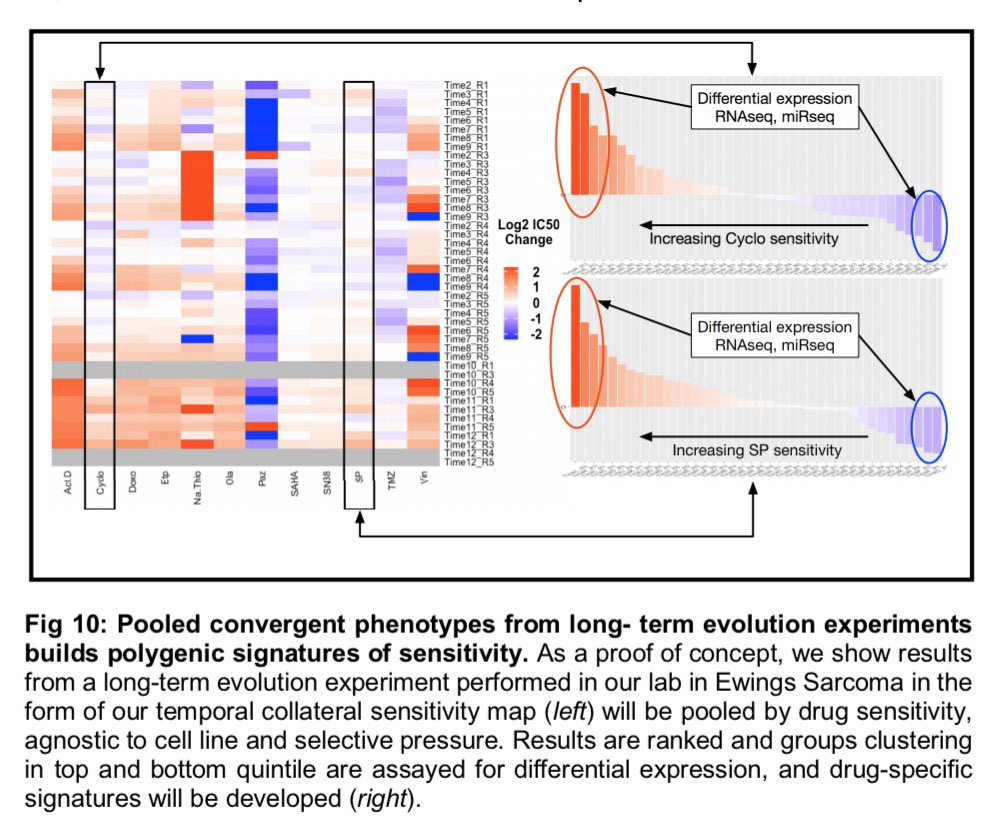
2nd aim will be to study commonalities in drug sensitivity/resistance - over a long (well - longish, not @RELenski long) term evolution experiment - how do sensitivities change and can we ID them? This will support super ⭐️ @CWRUSOM MSTP @ScarboroughJess -w/ help from @n8pennell. (this aim supported by our own work in E. coli).



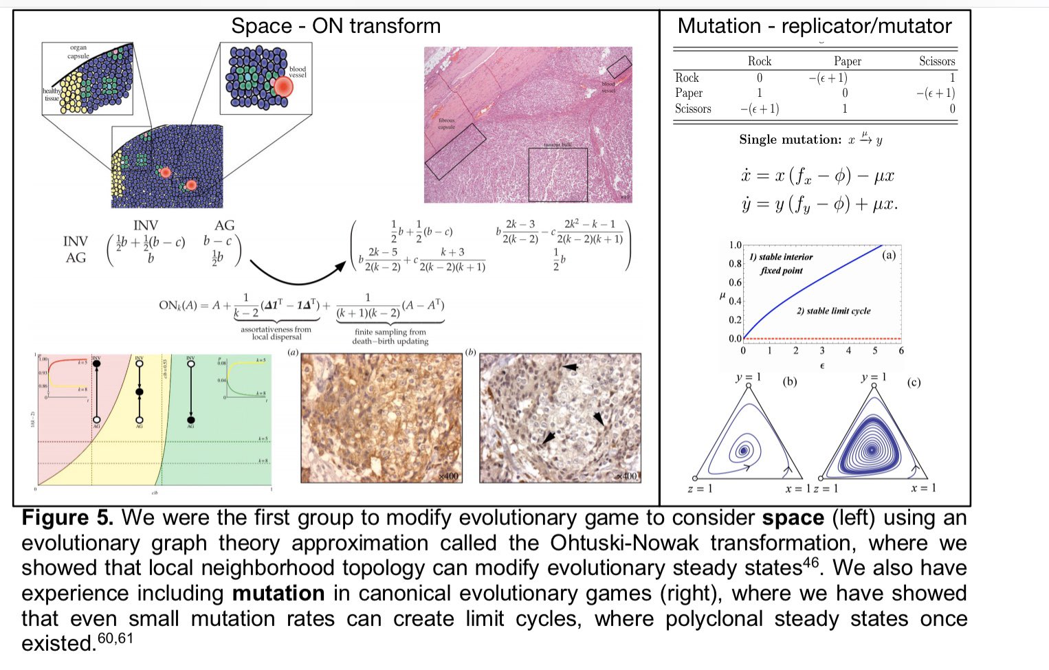
3rd aim will probe the evolutionary stability (in space (as we've done before on graphs) and time) of the ecological dynamics we measure in our game assays. Implementing replicator-mutator dynamics in collab w/ @stevenstrogatz
 - we’ll see how these games change through time. (h/t to @kaznatcheev for the idea!)



This also means that we are looking for someone to join the team...  specifically a postdoc with an interest in ecology and evolution and a desire to do some modeling and in vitro experiments. Cancer experience is NOT required, kindness and inclusivity are. Please spread the word or check out lab website and get in touch if interested by email.

Range expansion shifts clonal interference patterns in evolving populations

While Nikhil was trying to sort out a simulation of Michael Baym's beautiful megaplate experiment, we started wondering about the comparison of effective population size and agents in his (Nikhil’s) individual based model. The struggle was that to 'realistically' simulate this in a CA model would require order 10^10 agents, something that is not feasible. We were looking at something more like order 10^4... so what did that mean? Each CA element was something like 10^6 bugs? If that was the case -- what does 'mutation' mean in terms of our CA model?

Figure 1B from Baym's science paper (link above). The real size is on the order of feet...  that is a LOT of bugs.

What it would mean is that instantly, all 10^6 or so bugs would change their genotype... well, this was clearly crazy wrong :)

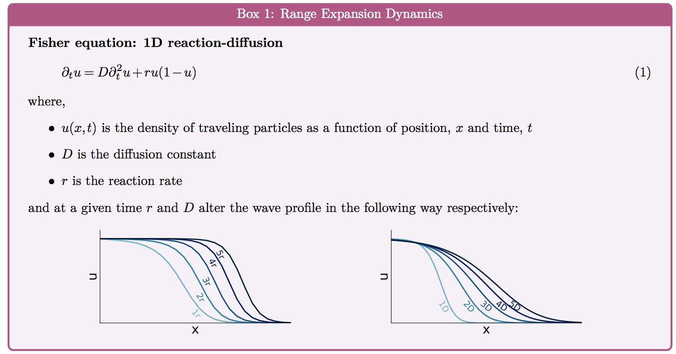
So, we started thinking about how populations spread in space (Fisher-like waves), and we found the wonderful body of work from the Gore, Hallatschek and Korolev labs thinking about mutational surfing (essentially at the wave tip there is a changed effective population size so the balance between drift and selection can change)

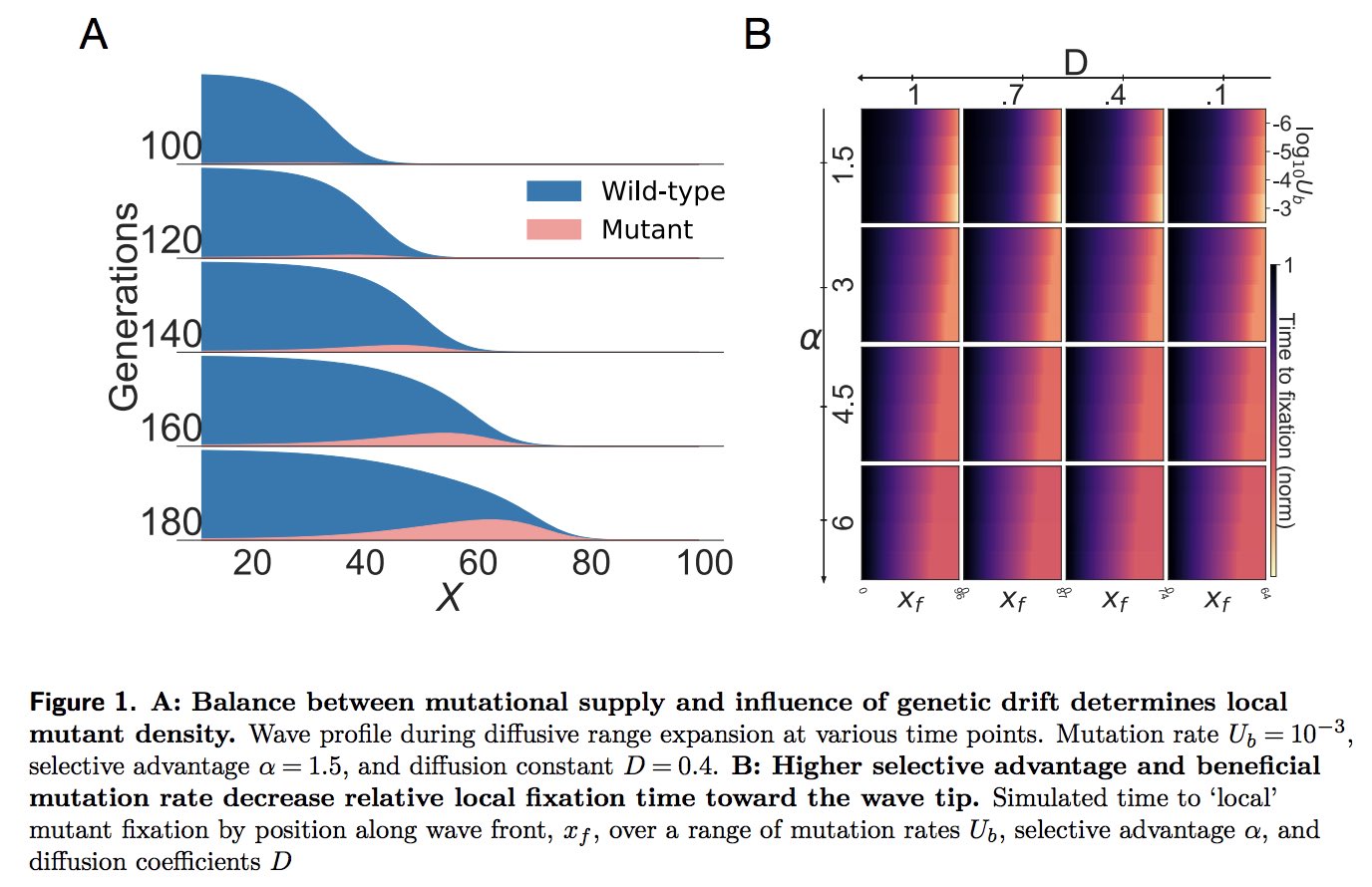
Formulating a model of (stochastic) mutation dynamics in a Fisher-like wave like those before us yielded known results. For a range of parameters, fixation of mutants can be promoted near the wave front - often called "mutations surfing on a wave".

So far, all this is known. Let's also recall from standard (well mixed) popgen (think Kimura) that depending on the relationship between the average time to establishment of a mutant, and the time to fixation, we can have qualitatively different evolutionary dynamics (e.g. strong selection weak mutation (SSWM) when the time to establishment is far larger than time to fixation; and weak selection strong mutation (WSSM) or strong selection strong mutation (SSSM) when the opposite is true, of if they are comparable). This is where we started to wonder...

we think a lot about strong selection (like in the form of experimental evolution in antibiotics or associated mathematical models of similar systems) and often make the assumption that our dynamics are in the SSWM regime -- but this need not always be the case (in fact, it likely isn't).

So, to really get at this, Nikhil defined a 'clonal interference index' as the log of the ratio of the fixation and establishment time, and calculated this all along the wavefront. What popped out is a pretty fun result: depending where are you on the wave front, you experience qualitatively different evolutionary dynamics.

This is our first real effort working in the range expansion space -- so we are very eager for any feedback (in particular if we've missed key references or if this is already a solved problem!).

Please check out the full preprint on bioRxiv for more details, and drop us a line if you have comments/questions.

The road to measuring evolutionary games in cancer

After I finished residency I actually wasn't able to negotiate for a full faculty job that had the parameters I was looking for (read: protected time, lab startup). But, I had worked for so long to get to the physician-scientist track that I wasn't willing to accept less than what I thought I needed to succeed.  This is something we can revisit in another post, but it sets the scene for this story, because what I did was take a sort of combination fellow/post-doc position where I trained. My two chairs, Sandy Anderson (Integrated Mathematical Oncology) and Lou Harrison (Radiation Oncology) were open minded and generous enough to create a position for me, so that I could get started on research that might lead me to be more competitive the next cycle.

This ended up being a super productive year, and led me to the job I now have (many thanks!). Also, during that year I met Andriy Marusyk, who is now my principle collaborator, and a close friend (sadly, not close in distance, but that's ok). Also during that year, Artem Kaznatcheev was working in Tampa with David Basanta, another friend and collaborator (and game theorist) of mine. At the time, Jeff Peacock was a 4th year medical student at UCF, and was rotating in my lab before starting his radiation oncology residency at Moffitt where I was (pseudo)faculty. During the course of that year, we had weekly discussion and brainstorming sessions, which were low stress, exciting times (Figure 0).

Figure 0. Artem, Robert and Andrew. Three awesome PhD students, discussing this project in what was likely the best office I will ever have.

David and Artem and I had been working for some time on evolutionary game theory (EGT) -- in the form of theoretical models. As a matter of fact, the first time we interacted with Artem produced a 96 hour hackathon and one of our most influential papers to date which I (and Artem) have previously blogged about -- an exploration of the effect of interaction neighborhood size on EGT dynamics (See Figure 1) - where we applied an algebraic transform on the game matrix to account for local interactions, derived from evolutionary graph theory, called the Ohtsuki-Nowak transform (more here on Artem's blog, or the original paper).

Figure 1. Taking a cartoon version of a tumor (upper left) and a prescribed (invented) evolutionary game to go with it (just below, left-most equation), we can transform the game to take into consideration the relative opportunities to interact with different types based not just on frequency, but also on location. This yields a somewhat messier game matrix (right-most equation), but also lets you explore how the dynamics will change with changing neighborhood size (lower left).

Andriy had just come off an exciting paper where he and colleagues explored an experimental model of breast cancer dynamics and showed that 'non-cell autonomous effects' (i.e. interactions) could change the overall composition of a tumor. In this paper, they used different fluorescent labels to track proportions of different types over time. This led our discussions to how we might be able to directly measure a game over time (there is a nice series of more technical blog posts by Artem which you can find referenced in the most recent in the series: here).

In addition to being ABLE to measure a game, we wanted to start with a situation which we thought would have a decent chance of also being interesting. We had just come off a project studying the changes in drug sensitivity over time of ALK mutated non-small cell lung cancer, and so had evolved TKI-resistant lung cancer cells lying around. We hypothesized (as most were at the time) that there would be a *cost* to the resistance, which we might be able to take advantage of in the form of a measurable *trade-off*. A quick and dirty first experiment that Jeff ran gave us some hope that this might be true (Figure 2).

Figure 2. We plot drug (Alectinib) dose on the x-axis, and optical density on the y-axis for three cell types, evolved Alectinib resistant H3122 (blue), drug sensitive H3122 (red) and Cancer Associated Fibroblasts (grey). We see that the higher fitness of naive cells at low drug dose switches to a lower fitness (relative to the resistant) at high dose.

We termed this result 'the cross' as our proxy for fitness (in this case optical density) *crossed* at a specific drug dose.  That is, after a specific dose, the most fit cell type changed from the wild type to the resistant, but critically, at low doses, we saw that the wild type was higher fitness than the resistant -- confirming our hypothesis (and bias) that at low drug concentration, being resistant *carried a cost* of lower growth rate. Interestingly, when we played this out in a different experimental system (measuring growth rate in a time lapse microscope), this fitness cost disappeared (see right-most two sub-figures in Figure 3).  I sometimes wonder if we would have continued with the experiment if we hadn't see this cost up front... 

Figure 3. Naive H3122 and evolved resistant to Alectinib (erAlec) cells grown in monoculture compared across four experimental conditions.

Anyways, by the time we measured the growth rates in Figure 3, Artem had already come up with a clever way to directly measure a game (which we assume to be a linear matrix game). By plating sensitive and resistant cells in a variety of proportions (ranging from 0:100 to 100:0) and measuring growth rate (proxy for fitness), then fitting a line, the intercepts would be the entries to the payoff matrix!  Figure 4 is the figure from the paper showing 4 different experimental conditions (with/without Alectinib and with/without Cancer Associated Fibroblasts (CAFs)).  It is a little busy, but it has ALL the info.  The inset plots are example shots of how we measured growth rate, by figuring out the total area of each (minor y-axis) red and green (sensitive and resistant) frequently over time (minor x-axis). Each of the individual proportion conditions are then plotted on the major axes with the opacity of the point telling what plated proportion were parental.

Figure 4. ALL THE DATA. Each experimental condition is a different color/shape as represented by the labelled convex hulls. Opacity is plating proportion of parental (1-resistant). The inset show how we obtained the growth rates, with example data points shown (green and red lines).

To explain how we get from here to a familiar appearing game notation, I'll 'blow up' one of the datasets (the Alectinib treated one - blue squares - in the far left convex hull).

Figure 5. Blowing up just the Alectinib treated cells, we can see how each data point in Figure 4 corresponds to a pair of points in the left sub-figure here (and the x/y axis in Figure 4). 

All the data points here are paired (80:20 etc), and the pairs (vertically aligned) match up to a single point in the previous figure. You can see here that we then perform a linear fit, which we can now use the intercepts to derive the payoff matrix elements, like this:

Figure 6.  We can now see how the intercepts of these lines forms the entries into the familiar payoff matrix.

Now we have a familiar payoff matrix!!  We can then plot the payoff matrix in a game space (which Artem nicely explains on his blog here), and compare the experimental conditions -- and we see that the DMSO+CAF game is qualitatively different than the others (Figure 7).  A cool result on its own. The canonical games represented are 'Leader' and 'Deadlock' - games which have not received much (any) attention to date in the oncology-EGT literature.

Figure 7 - some future directions/food for thought...

Another fun thing we noticed is that it appears that each perturbation (drug/CAF) shift the game in a particular way (see cartoon versions of vectors representing these changes in the game in red and blue). We haven't fully explored this yet, but it is thought provoking...

Taken together, we have a new assay, which we hope more folks use to measure a catalogue of games played by other cancer types, and a new way to perturb evolution -- by treating the game instead of the player. The central focus of our lab is exactly this: to get control of/take advantage of the evolutionary process on the way to resistance.  While this assay, and the resulting measured game, takes place over a short time-scale (5 days), it does give some insight into some new ways to pick/bias the winner in a low complexity game. We are hoping to extend the assay to more strategies to better represent more complex tumors, and also to think about longer timescales -- this will require not just new experimental technique, but some new theory as well. Further, this theory fits in well with the work on collateral sensitivity which we recently reported in E. coli with Dan Nichol as lead author... though that work is the opposite end of the time-scale spectrum (relatively very long time scales - actually infinite time in the theoretical work, but ten-days in the experimental work, which for bacteria is MUCH longer than the 5 days in cancer cells here).

Anyways, the work continues! For more information on measuring games, check out the full paper: 

Fibroblasts and alectinib switch the evolutionary games played by non-small cell lung cancer 

published last week in the journal Nature Ecology and Evolution, along with an associated editorial which describes a bit more about evolutionary therapy.

Antibiotic collateral sensitivity is contingent on the repeatability of evolution

You know those moments when you read a paper and your head just explodes?  It's happened a few times to me in my life, and when it does the whole moment gets seared into my head.  One of those moments happened on a spring day in Oxford. I was eating a bap I had bought at the Taylor's expansion (1) by the old math's institute on Little Clarendon, sitting by a war monument (2). Here:

What I read was a paper from Dan Weinreich called Darwinian Evolution Can Follow Only Very Few Mutational Paths to Fitter Proteins. In this paper they engineering 2^5 = 32 strains of E. coli with 5 different basepair substitutions in a gene that encodes resistance to a certain kind of antibiotics. Then they simply measured the fitness of each of the strains, and constructed a hypercube, like Sewall Wright suggested first in 1932 (before anyone knew anything about genes!  he just called them allelomorphs).  If you make a 5-cube, like Wright sketched:

If every mutation gives you a fitness boost (as the literature showed they individually do) you should be able to get from wildtype (far left) to 'fully mutated' (far right) in 120 different ways. This would be something called a Mt. Fuji landscape, with one peak.  All paths go 'up' - which is essentially the null hypothesis that this paper was testing. At the time, I hadn't thought much about any other possible concepts -- being taught from the clinical oncology more-mutations-is-bad canon -- the more mutations a cancer has, the worse (more fit) it is.  (n.b. we can talk a lot about different 'kinds' of mutations - like passengers vs drivers, some other time, and also there's the whole fact that mutational effects are likely context dependent -- but we'll get to that later). Anyways, this is where the hair on fire part came for me. After they measure all the corner's fitnesses, they found that only 18 paths existed to get from left to right - and showed this figure:

There I sat, with my hair on fire, and a bap dangling out of my mouth. My world had changed forever.  What they showed here was empirical proof that the theoretical possibility that some combinations of mutations (even if they are individually beneficial) can be deleterious!  That means to two beneficial mutations could add up to a fitness penalty. This is something called epistasis (actually it's a special type called reciprocal sign epistasis, which you can read more about here).  While this was known to other members of the scientific community, it was not to me, and this set of a bunch of thinking that led to the idea that Dan Nichol and I (and friends) explored in our 2015 paper Steering Evolution with Sequential Therapy to Prevent the Emergence of Bacterial Antibiotic Resistance. Here, we used a set of fitness landscapes that were measured in a similar way to the above description, but for a lot of drugs, that were published by Mira et al. together with a mathematical model that Dan came up with.

This model is a time homogeneous absorbing Markov chain model of evolution that requires assumptions about the population all being on a single corner of the hypercube at any given time (often referred to as Strong Selection Weak Mutation (SSWM)).  Dan then calculated the probability of any given mutation from corner i to corner j ($P_{ij}$) based on changes in fitness from one corner to the next, like this:

Using this, and some matrix multiplication, we came up with the cute idea that evolution doesn't (necessarily) commute - that is, the evolutionary outcome could be quite different if you applied drug A and then B, as opposed to drug B and then A.

Given that many of the landscapes have more than one peak, there are also a number of situations in which evolution has to make a choice... it can go uphill in more than one direction. You can visualize this like a series of hills in which the population is 'walking up' them.  Given that the population can't 'see ahead' but can only make decisions about going 'up' instead of 'down', you can imagine that a population could easily evolve to an optima that is not globally optimal. You can see an example below (in panel (a)) where a strain starting at the yellow circle would move uphill to the blue triangle and then have to choose 'left' or 'right'. (obviously the geometry of this is wrong, but it is the best we can do as humans to visualize)

A few things become clear - one is that the fitness through time would be different (as you travel different trajectories even going 'up', it could be different along the way), and the other is that the end fitnesses will also differ (if you believe that evolution will EVER find a peak, which Artem doesn't -- more here in his bioRxiv preprint or on his blog).  AND if you then consider the end position, and how it relates to fitness IN ANOTHER LANDSCAPE (see panel (b), above for a visual representation), you have a situation where the outcome of drug sequencing can change with the evolutionary 'decision' - or in our jargon collateral sensitivity changing depending on evolutionary contingencies.

This led us to want to do the experiments. So, we continued our collaboration with Robert Bonomo at the Cleveland VA hospital, and performed 60 replicates of the same experiment - 60 what we now term evolutionary replicates. Just showing the first 12, we see evidence for the different trajectories encoding different fitnesses through time, here:

Out of curiosity, we wondered how common it would be to get a different answer to the question: If I give one drug (drug A) and then another (drug B), how much variation could I see in collateral response. To answer this, we used another version of the mathematical model from our first paper (which you can download here, along with the data needed to redo our analysis). It turns out that there is wide variability in collateral sensitivity (according to our mathematical model), so much that any one repeat of an evolution experiment could give you an opposite answer (could reveal collateral sensitivity) when the very next one could reveal cross-resistance.

This is sorta bad news...  but to try to find the bright side, we propose using a new metric, which we call Collateral Sensitivity Likelihood (CSL), which is a measure of a sequence of drugs providing any collateral sensitivity at all.  This would make for safer recommendations -- where what you want is some method for clinicians to rationally choose a drug ordering that has a high probability of being better (or the opposite, a low probability of the drugs inducing resistance to one another).

So - from hair on fire to 5 years of research later, we finally were able to get this story out there. We published it last week, and you can read the whole paper, which is open access, here: Antibiotic collateral sensitivity is contingent on the repeatability of evolution.  Lots more details and figures are available there...

In addition to making the code and phenotype data available (in the embedded github repo link), we also performed whole genome sequencing on 12 of the evolutionary replicates, and we uploaded those data to the NCBI Sequence Read Archive (SRA), and they are freely available through accession code PRJNA515080, or through this link. So, hurray for #openscience - we'd love any secondary analyses or ideas for future projects.  Lots to think about.

If this research interests you, please check out our lab page to see what else we're up to.  We're trying to apply evolutionary thinking, mathematical models and experimental evolution to cancer and pathogens to ease suffering.